New Old Approach to Dynamic Range

Preamble

In today's world, "dynamic range" (DR) has become, in the minds of (many) photographers one of the main characteristics of a digital camera.

Unfortunately, the public data on DR is limited to "DD - ISO sensitivity" graphs and tables. This can be "engineering DR", EDR, like for DxO Mark, meaning that the signal/noise ratio, SNR, is equal to one; or this can be "photographic DR", PDR, like Bill Claff provides here, setting a higher boundary for S/N ratio. With this, the nature of noise (for example, random noise, banding) isn't accounted for, however the noise character is important for visual quality.

In certain cases, anomalies can be found in DR databases, the interpretation of which requires a somewhat deep understanding of where they came from.

Furthermore, measuring DR by the noise in the shadows doesn't account for the possible processing of the signal in the camera. In part, if there is noise reduction or bit depth reduction taking place in the camera, then the level of noise will be (relatively) low, but that very same noise reduction will destroy small low-contrast (and sometimes not so low) details.

In reality, any practicing photographer knows that the degradation of the image in the shadows (or because of low exposure) happens gradually, there is no strict demarcating line. It's just that with the lowering of exposure, small details disappear, the contrast between bigger details diminishes, color fidelity becomes worse. Depending on the quality demanded of the image (which will depend on presentation size, viewing distance, other viewing conditions such as screen resolution, etc.,), the practical dynamic range for the specific camera will be different, even for the same ISO setting.

What we used previously (Old Approach)

Four years ago, while studying a newly-bought Canon EOS 6D, we tried to approach the program of practical dynamic range in the following way:

• A target with known contrast (gray text on a gray background with contrasts of 0.5, 1, 1.5 EV)
• and with details of known size was photographed (12pt, 18pt, 30pt font);

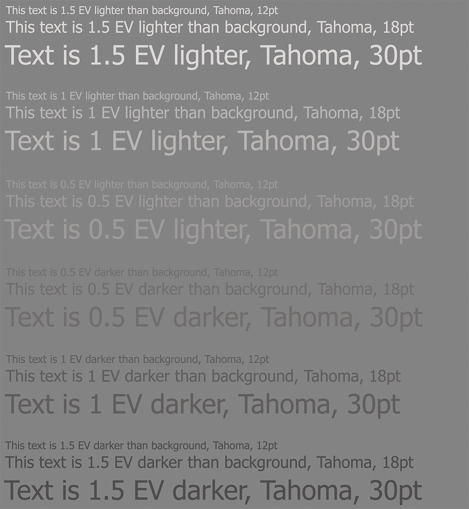
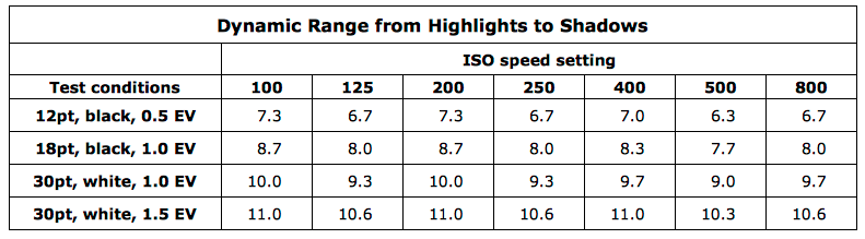
The practical boundary of the dynamic range was set by the legibility of the letters with fixed size and contrast ("12pt with a contrast of 0.5EV is legible" - can be zoomed in, and viewed in large format; "30pt with a contrast of 1.5EV is legible" - can be published online). The real "working DR" data spread was, for EOS 6D and ISO 200 from 7.3 stops by the strictest criteria to 11 stops by the loosest.

Illustrating our current method (New Approach) using Canon 5D Mark IV

The concisely-described above-mentioned "old method" allows one to consciously set the upper and lower limits of the working dynamic range of the camera, but it doesn't give information about what's happening within that range. One could increase the range of letter sizes by adding in smaller letters, or one could do otherwise:

• Let's take, for example, a part of the standard ISO 12233 target,
• But let's print it at low contrast,
• And how about on a weird tilt, so the clever algorithms that are there to restore horizontal/vertical lines (if the camera has them) break.

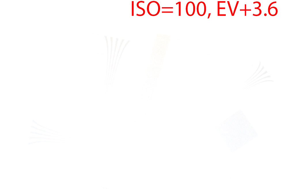
For example, something like this (this is a real shot of a real target, click to see a bigger version):

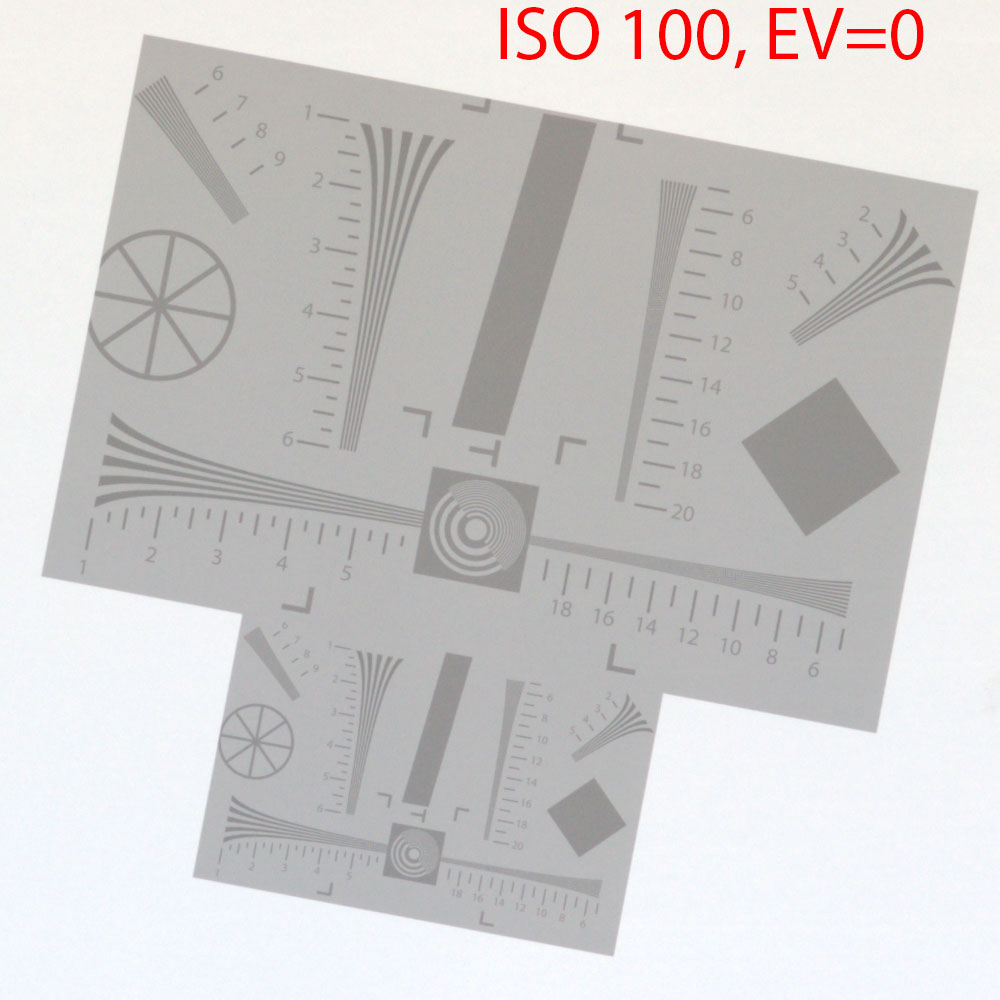
0. Some necessary explanations:
1. Here are two resolution targets that differ by a factor of 2 in size, since during the preparation stage it was unclear which size would be optimal (from now on, we will be using the larger, upper target illustration).
2. EV = 0 - the exposure that is used is such that the gray background of the target in the RAW was at 12.7% of the clipping level: 3 stops below clipping is the current generally-accepted place for middle gray in RAW, coming from the idea that 2.45 stops (18%) is obviously too little in practice, 4 is a bit too much, and we'd still like to have a nicely rounded value (to get exactly -3 EV, 12.5% should be used, log2(0.125) = -3; however 0.5 EV down from 18% is 12.7%, making it easier to compensate the exposure when a standard 18% card is used).
3. For this and all following examples, the RAW has been rendered in 1:1 scale, shots were taken with a Zeiss Makro Planar 100/2 lens set to f/8, the target was in the center of the shot at a distance of 3.5 meters, with the entire shot of the target fitting into a 1000x1000 pixels square.

If you take a picture of this target, bracketing the exposure using the shutter speed (at the same aperture and ISO speed setting) and then (within reasonable limits) compensate for exposure ("pull the shadows back into middle gray") then we will see the following:

Shadows

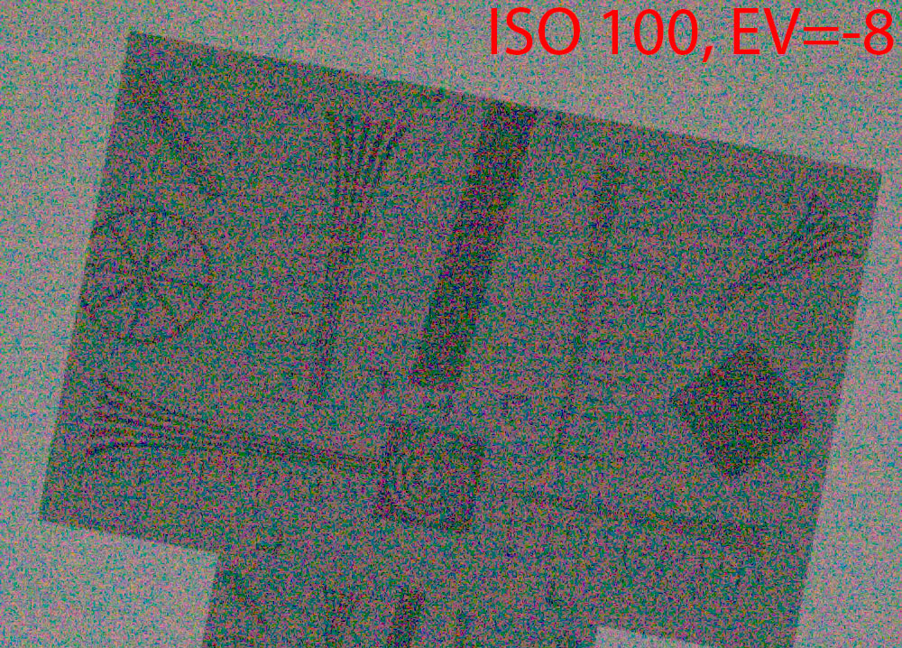
Here are four shots (to see them full-sized, please click)

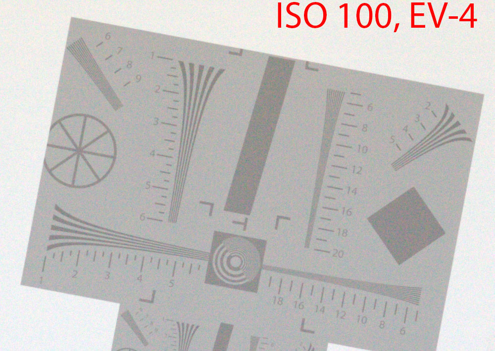
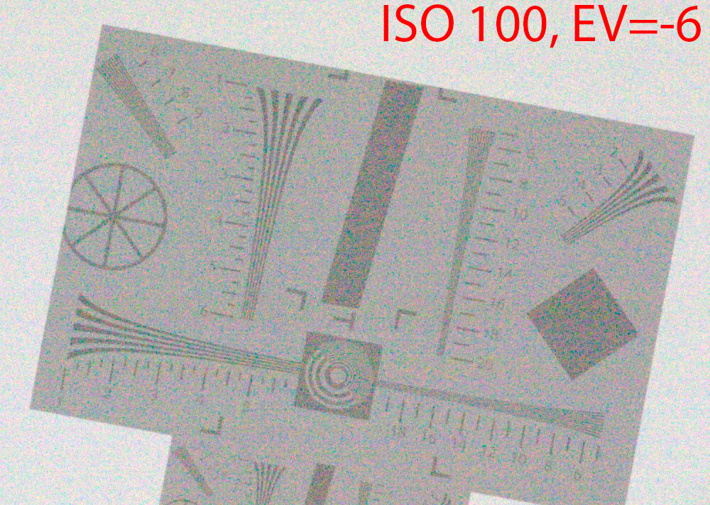
• As it is easy to see, when exposure decreases (this can be the shadows on a normally-exposed shot, or middle gray on an underexposed one), the resolution falls gradually and steadily:
• -4 EV below middle gray - the resolution has fallen by about 20% (at the shot whee EV = 0 the dashes were read around the 10 scale mark region, for EV = -4, around the 8 scale mark)
• -6 EV - the resolution falls by a factor of two from optimal exposure
• -8 EV - the resolution falls by a factor of four
• -9.6 EV - in practical terms, it's fallen to zero - only the very large, 100-pixel objects are somewhat visible.

There's nothing unexpected here - first the resolution falls gradually, then quickly.

Highlights

In the highlights, the situation is a bit more complicated than it can be supposed, because in vast majority of cases only the linear portion of the characteristic curve of digital image sensor is used in consumer cameras (there are a few exceptions to this rule, like some Panasonic cameras at lowest "actual" ISO setting).

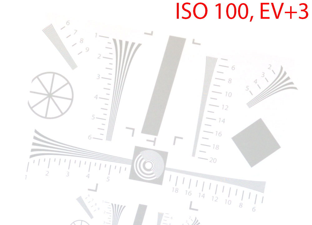
The gray background has become completely white (which is completely predictable, EV = 0 corresponds to a level of gray 3 stops below clipping; accordingly, with +3 EV exposure we get to clipping). However, the darker lines are all in place and the resolution is also there.

However, if we increase the exposure by another 0.6 stops, only the biggest details in the scene will remain, and even they aren't that visible:

The reason for the disappearance of small details (the contrast of which relative to the background is the same as for large ones) may be not obvious, but it is interesting. Let's look at a histogram of the black square in the right part of the shot:

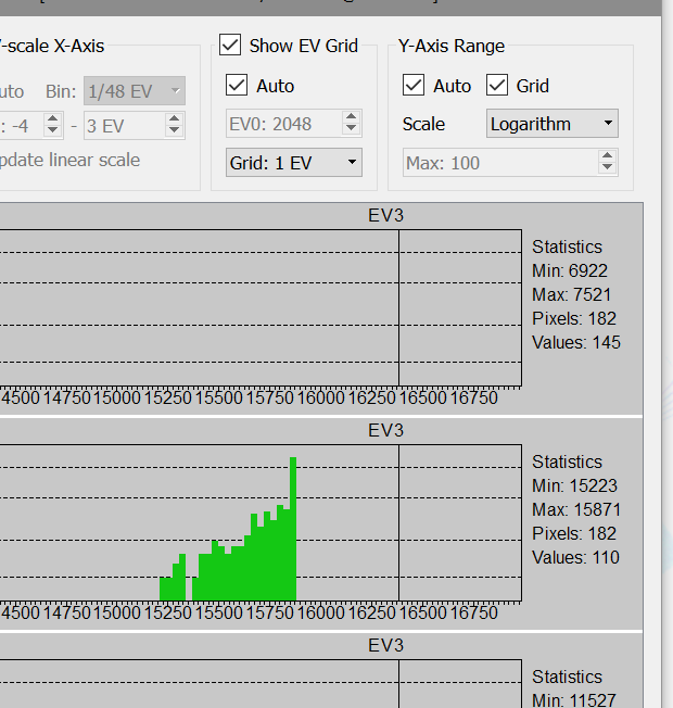
As we remember, photon flow always has some scatter (photon shot noise, the noise associated with the random arrival of photons on the sensor; "variance equals signal"), as a result the histogram of the single-tone objects is shaped like a bell. On the shot being looked at, the bell on the dark objects is such that its edge has ended up being below the level of clipping. On large objects, this is enough to display them. On smaller ones, there aren't enough pixels, the bell isn't wide enough, it doesn't get past the edge, and there are too few pixels darker than the clipping point to create a visible image.

Results and Analysis

In practice, resolution is evaluated using a semi-automatic computerized method, while the target shots (analogous to the ones shown above) were used for selective verification by eyeballing.

The results are shown on the following graph:

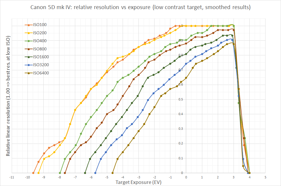
• On this graph:
• The horizontal axis - the exposure of the target, 0 corresponds to "middle gray" (at a level of -3 EV from clipping in the green channel), accordingly everything that's in the positive part (right) is the scene's highlights, everything that's in the negative is shadows.
• On the vertical axis - the relative resolution, 1.0 is taken as the maximum possible resolution on low ISO.
• The precision of this vertical axis is around 0.05-0.08 units (5-8% of resolution) or about one small division, so one need not treat these graphs as absolutely precise.

0. Looking at this graph, we can see a lot. For example:
1. At ISO 100, at the level where "resolution is just a bit higher than zero" we get a dynamic range of 12 (up to 13) EV. Only the real resolution at the boundaries of that range will not be in megapixels, but in kilopixels (see above example at -9.6 and +3.6 EV), some large objects will be somewhat visible over the noise on the background.
2. ISO 200 and ISO 100 basically cannot be told apart on this camera, which is completely normal for Canon cameras.
3. If, on low ISO, one underexposes a couple stops (meaning that instead of EV 0, end up at EV -2), and then pull out that exposure in a converter, that will lead to a loss of 10% by linear resolution (meaning that a 30-megapixel camera will become ~24-megapixel).
4. If, instead of ISO 200, one sets ISO 400 and exposes optimally, then this will lead to the exact same effect: a loss of 10% in linear (and ~20% in megapixel) resolution.
5. Further increases of ISO speed lead (with correct exposure) to further losses in resolution in the middle gray, and at ISO 6400 we have about a 12-megapixel camera (instead of 30Mpix).

One can use the graph in a different manner as well: choose some resolution value which interests us. Let's say 3840 on the long side - this is 0.57 from the (formal) camera resolution.

• Let's draw a horizontal line at the 0.6 level and see that with the selected resolution loss, we will have the following DR:
• 8.6 EV (5.6 in the shadows, 3.0 in the highlights) for ISO 100-200
• 7.5 EV for ISO 400
• 2.7 EV for ISO 6400, but all of this DR is in the highlights and if we want to use them somehow and get a good shot for a 4K monitor, then we'll need to turn the exposure correction positive (so killing the "room in the highlights").

The camera only gives full resolution at ISO 100-400 and in the highlights (this, by the way, explains why ETTR is good).

In general, all of this analysis is banal and completely follows from the graphs.

The only non-banal conclusion that we can formulate is this:

• Let's suppose that we have a fast lens (for example, f/2) whose optimal diaphragm in terms of image quality is (again, for example) f/5.6
• We're shooting a dimly-lit scene and want to increase the ISO (and shoot at "optimal diaphragm" since it's optimal).
• Well, it turns out that it may be much more worth it to not increase the ISO, but rather open up the aperture a bit more than optimal: the losses in resolution due to suboptimal diaphragm may turn out to be lower than the losses due to increased ISO.

P.S. The underexposure in these tests was due to increase of the shutter speed, and the data for the extreme left points on the X axis was obtained at very short exposure, down to 1/8000 sec. In real life, the situation will be worse (the noise will be higher, and the DR will be correspondingly lower) due to additional heat noise on real (much longer) exposure.

P.P.S. On other cameras, the exact numbers will be different, but the general look of the graphs will remain because the "noise at high ISOs" (at reasonable exposures, less than a second) is the noise from the signal itself (photon shot noise), not the noise from the camera's electronics.